This example looks at anticipated precision for a potential CKMR study patterned after the biology of beluga whales in Alaska. I initially developed this while attending a workshop Mark Bravington gave looking at the potential for CKMR for assessing various Alaskan terrestrial and marine mammal populations. Not having access to individual-based simulation software, my initial attempts used expected numbers of kin pairs (using relative reproductive output calculations) to simulate data. This initial code, programmed entirely in R, is located here.
In this example, I extend this example to use individual-based simulation using the CKMRpop package [1], writing pseudo-likehoods in R. Let’s start by downloading the CKMRpop package and installing relevant libraries in R (note that you also need to have previously installed RTools). For further help with CKMRpop installation and example simulations, see here.
remotes::install_github("eriqande/CKMRpop")
library(CKMRpop)
library(dplyr)
install_spip(Dir = system.file(package = "CKMRpop"))
Now, let’s try setting up simulations with a life history resembling a beluga whale population. Note the quotation list structure is required by CKMRpop, and that the package is set up to work with a post-breeding census. For definitions of the pars list, please use spip_help() or spip_help_full(). Here are some life history schedules:
pars <- list()
pars$`max-age` <- 40  #high survival so need to run for quite a while to kill everyone off
pars$`fem-surv-probs` <- pars$`male-surv-probs` <- c(0.7, 0.95, rep(0.97,38))
pars$`fem-prob-repro` <- c(rep(0,6),c(.2,.4,.6,.8),rep(1,30)) #probability of reproduction *if* no current calf
pars$`repro-inhib` <- 1  #no repro if calf is 0-1 year old
pars$`male-prob-repro` <- pars$`fem-prob-repro`
pars$`fem-asrf` <- rep(1,40)  #if they reproduce, they will have at most 1 offspring
pars$`male-asrp` <- rep(1,40)  #each reproductively mature male has same expected repro output
pars$`offsp-dsn` <- "binary"  #override default neg. binomial dist. for litter size
pars$`sex-ratio` <- 0.5
Now we’ll set up some initial conditions and specify the length of the simulations. We’ll base the age structure of founders on stable age proportions computed using Leslie matrices, as calculated via the leslie_from_spip functionality in CKMRpop:
pars$`number-of-years` <- 140
# this is our cohort size
cohort_size <- 300
# Do some matrix algebra to compute starting values from the
# stable age distribution:
L <- leslie_from_spip(pars, cohort_size)
pars$`initial-males` <- floor(L$stable_age_distro_fem)
pars$`initial-females` <- floor(L$stable_age_distro_male)
pars$`cohort-size` <- "const 300"
Note that when the cohort size argument is set to a constant, that the implied fecundity values in the Leslie matrix are rescaled so that the finite population growth rate, \(\lambda\), is 1.0. This can be useful for simulation, but may make comparing fecundity values estimated by a CKMR model to those used to simulate the data difficult (although fecundity-at-age curves should be proportional). If this feature isn’t desired, CKMRpop can also be run with time-specific cohort sizes, or fishsim can be used for simulation.
Next, we need to specify how the population is sampled. For simplicity
samp_start_year <- 121
samp_stop_year <- 140
pars$`discard-all` <- 0
pars$`gtyp-ppn-fem-post` <- paste(
  samp_start_year, "-", samp_stop_year, " ",
  paste(rep(0.01, pars$`max-age`), collapse = " "),
  sep = ""
)  #basically we're saying that beluga hunters aren't biased towards a particular age class, and that we're sampling 1% of the pop per year - about 30/year
pars$`gtyp-ppn-male-post` <- pars$`gtyp-ppn-fem-post`
In CKMRpop, we need to include enough time so that all sampled animals have grandparents, so we need to run the simulations for three generations before sampling is conducted. Let’s call spip to simulate the data, get results back into R, and make some summary plots
set.seed(2020)  # set a seed for reproducibility of results
spip_dir <- run_spip(pars = pars)  # run spip
slurped <- slurp_spip(spip_dir, 2) # read the spip output into R
ggplot_census_by_year_age_sex(slurped$census_postkill)
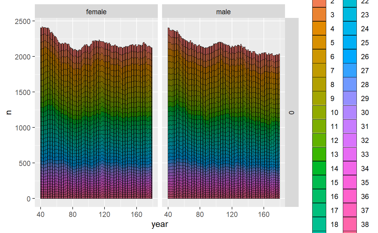
Okay, now we have a virtual population. There are many other ways that CKMRpop has to visualize simulation results (which are worth looking at!), but for a scoping study the next thing we want to do is to start looking at sampled animals and number of kin pairs to make sure they line up with what we were hoping.
So, after 20 years of sampling (at an average of 40.15 samples per year), we end up with 803 tissue samples. Assuming none are corrupted (a dubious assumption), they can be genetically analyzed and kin relationships can be determined. CKMRpop actually keeps track of a lot of relationships - more than are needed for CKMR analysis (at least in CKMR’s current state). Nevertheless, they can be useful because they can allow us to examine the performance of CKMR estimators when there are errors in kin determination (e.g., grandparent-grandchild or aunt-niece being mistaken for half-sibs). Here is a summary of true kin-pairs in our sample:
relat_counts <- count_and_plot_ancestry_matrices(crel)
relat_counts$highly_summarised
# A tibble: 5 x 3
  dom_relat max_hit     n
  <chr>       <int> <int>
1 FC              1   642
2 A               1   453
3 Si              1   178
4 PO              1   120
5 GP              1    69
So, there are 642 first cousin pairs, 453 half-avuncular pairs, 178 half-sibling pairs, 120 parent-offspring pairs, and 69 grandparent-grandchild pairs. So, if we’re interested in conducting an abundance analysis with parent-offspring pairs, we should have enough data to come up with a decent estimate, although this likely depending on how much flexibility we want with modeling population trends and how precisely harvested whales can be aged. If we’re going with half-siblings, we’d want to take special care to limit comparisons to a time range (e.g., those with ages within ten years of each other) to prevent contamination with grandparents (we will not usually be able to tell these apart genetically). This can present some serious problems if ages (or a good proxy) aren’t available!! If good age estimates weren’t available we might just want to limit half-sib comparisons to calves within a a reasonable time frame (e.g., calves harvested between 2 and 10 years apart). Alternatively, we might try to model kin pairs which ``look like half-sibs" as a mixture of grandparents and true half-sibs, using simulation to guide what the mixing proportion should look like. Ugly, but perhaps possible.
One thing worth mentioning is that running CKMRpop with spip is currently set up for live samples, meaning that it is possible for animals to be sampled more than once and for adults to have offspring after they are sampled. This is opposed to fishsim which by default only samples newly dead animals. However, precision calculations shouldn’t be greatly affected since sampling probabilities are fairly low in this case.
The next step in actually using these simulated data to investigate anticipated precision of CKMR estimators is to get them into a format amenable to analysis. For simplicity, let’s assume that we’re just going to be modeling POPs. We’ll assume that sex is known and look at a model where age is assumed to be known with certainty. The sufficient statistics for such a model consist of the number of comparisons of different types, \({\bf n}\), as well as the number of those comparisons that result in kin pairs, \({\bf y}\). Both collections of statistics can be indexed by three subscripts: the year of the potential offspring’s birth (\(t\)), the age of the potential parent in year \(t\) (\(a\)), and the sex of the potential parent (\(s\)). Note that we’re going back to year 81 of simulation time as the start of the CKMR time series (beginning year of sampling minus one generation).
PO_only <- crel %>%
  filter(dom_relat == "PO")

y_tas = array(0,dim=c(60,40,2))  #CKMR sufficient statistics
#dimensions are year of offspring birth, age of parent in
# year of offspring birth, parent sex
for(i in 1:nrow(PO_only)){
  FIRST = (PO_only$born_year_1[i] < PO_only$born_year_2[i])
  # case 1: parent is animal 1
  if(FIRST){
    p_age = PO_only$born_year_2[i]-PO_only$born_year_1[i]
    p_sex = (PO_only$sex_1[i]=="M")+1  #1 for female, 2 for males
    o_by = PO_only$born_year_2[i] - 80  #year 81 in simulation = year 1 for CKMR inference
  }
  else{
    p_age = PO_only$born_year_1[i]-PO_only$born_year_2[i]
    p_sex = (PO_only$sex_2[i]=="M")+1  #1 for female, 2 for males
    o_by = PO_only$born_year_1[i] - 80  #year 101 in simulation = year 1 for CKMR inference
  }
  y_tas[o_by,p_age,p_sex] = y_tas[o_by,p_age,p_sex] + 1
}
Here, y_tas holds the number of matches of each type; we also need to know something about the number of comparisons that are made of each type to calculate a pseudo-likelihood. This is potentially very computationally intensive since there are close 3.22003^{5} comparisons to be made. This number goes up exponentially with sample size, so the following brute force approach will need to be improved for larger numbers of samples.
n_tas = array(0,dim=c(60,40,2))  #CKMR sufficient statistics
n_indiv = nrow(slurped$samples)
for(i1 in 1:(n_indiv-1)){
  for(i2 in (i1+1):n_indiv){
    born_diff = slurped$samples$born_year[i1] - slurped$samples$born_year[i2]
    if(abs(born_diff)<41){ #max age is 40 so don't compare differences older than that
      if(born_diff<0){ #first animal is older
        p_age = -born_diff
        p_sex = (slurped$samples$sex[i1]=="M")+1  #1 for female, 2 for males
        o_by = slurped$samples$born_year[i2] - 80  #year 81 in simulation = year 1 for CKMR
        n_tas[o_by,p_age,p_sex] = n_tas[o_by,p_age,p_sex] + 1
      }
      else{
        if(born_diff>0){ #note no comparisons for animals born in same year
          p_age = born_diff
          p_sex = (slurped$samples$sex[i2]=="M")+1  #1 for female, 2 for males
          o_by = slurped$samples$born_year[i1] - 80  #year 81 in simulation = year 1 for CKMR
          n_tas[o_by,p_age,p_sex] = n_tas[o_by,p_age,p_sex] + 1
        }
      }
    }
  }
}
So, not including comparisons where individuals are born in the same year or greater than 40 years apart, we have a total of 3.08623^{5} comparisons.
Now, let’s fit a CKMR model for PO pairs to these data. We’ll see how well we do at reconstructing population trend and absolute numbers. First we’ll write a negative log-pseudo-likelihood function. Note that since we have age-specific fecundity vectors, we’ll need to model age structure in order to calculate relative reproductive effort. We’ll do this by writing a model for adult abundance and passing in the expected age structure as “data.” Specifically, let’s assume an exponential model for abundance of ages 6+ (when animals start reproducing; we’ll call this “adult abundance”): \(N_t = N_0 \exp(rt)\). Here, \(N_0\) is adult abundance in year 1 (year 81 of simulation time) and \(r\) is the intrinsic rate of increase. Then, sex- and age specific abundance can be modeled as \(N_{t,a,s} = 0.5 N_t \pi_a\), assuming a 50/50 sex ratio. The proportion of animals in each age class is given by \(\pi_a\), where \(\pi_a \propto [1, S, S^2, \ldots]\) (it is then normalized to sum to one). We’ll assume that survival is known and will set it to it’s true value (0.97). If this were a comprehensive study, we’d want to explore ramifications of uncertainty (or ideally try to estimate it with a combined POP / HSP analysis).
log_p <- function(p){  #function to prevent errors with log(0)
  log(p + (p==0))
}


nll <- function(pars_CKMR,data){
  jnll=0
  rem_tas = data$n_tas-data$y_tas
  N_t = 500+exp(pars_CKMR[1] + pars_CKMR[2] * c(0:(data$n_t-1)))  #time specific abundance of 6+
  # note intercept so optimizer doesn't get weird rel_repro values
  N_ta = matrix(0,data$n_t,data$n_a) #same for males and females
  for(it in 1:data$n_t)N_ta[it,]=0.5*N_t[it]*data$Pi
  Repro_male = Repro_fem = Rel_repro_male = Rel_repro_fem = 0*N_ta
  for(it in 1:data$n_t){
    Repro_male[it,] = data$fec_male * N_ta[it,]
    Repro_fem[it,] = data$fec_fem * N_ta[it,]
    Rel_repro_male[it,]=data$fec_male/sum(Repro_male[it,])
    Rel_repro_fem[it,]=data$fec_fem/sum(Repro_fem[it,])
  }

  Log_rrm = log_p(Rel_repro_male)  #vectorizing before LL computation
  Log_rrf = log_p(Rel_repro_fem)
  Log_rrmc = log_p(1-Rel_repro_male)
  Log_rrfc = log_p(1-Rel_repro_fem)
  #females
  for(it in 1:data$n_t){
    for(ia in 1:data$n_a){  #product binomial likelihood w/o normalizing constant
      if(data$n_tas[it,ia,1]>0)jnll = jnll - data$y_tas[it,ia,1]*Log_rrf[it,ia] - rem_tas[it,ia,2]*Log_rrfc[it,ia]
    }
  }

  #males
  for(it in 1:data$n_t){
    for(ia in 1:data$n_a){
      if(data$n_tas[it,ia,2]>0)jnll = jnll - data$y_tas[it,ia,2]*Log_rrm[it,ia] - rem_tas[it,ia,2]*Log_rrmc[it,ia]
    }
  }
  #cat(sum(data$n_tas[,,1]*Rel_repro_fem) + sum(data$n_tas[,,2]*Rel_repro_male))
  return(jnll)
}
Okay, let’s put together our data and parameters and use nlminb to minimize the objective function.
  pars_CKMR = c(log(3700),0) #initial values for log(adult abundance), r
  Pi = rep(1,34)
  for(ia in 2:34)Pi[ia]=Pi[ia-1]*0.97
  Pi = Pi/sum(Pi)
  data = list(y_tas=y_tas[,7:40,],n_tas=n_tas[,7:40,],fec_male=pars$`male-prob-repro`[7:40],
              fec_fem=pars$`fem-prob-repro`[7:40],n_a = 34, n_t = 60, Pi = Pi) #note we're only modeling adults here so n_a = # of breeding age classes
  nll(pars_CKMR,data=data)
[1] 1024.431 Opt = nlminb(pars_CKMR,nll,data=data)
  Adults = rep(0,60)
  for(iyr in 81:140)Adults[iyr-80]=sum(slurped$census_postkill$female[which(slurped$census_postkill$year==iyr & slurped$census_postkill$age>6)])+sum(slurped$census_postkill$male[which(slurped$census_postkill$year==iyr & slurped$census_postkill$age>6)])
  Ests = 500+exp(Opt$par[1])*exp(Opt$par[2]*c(0:59))
  plot(Ests,ylim=c(0,5000))
  lines(Adults)
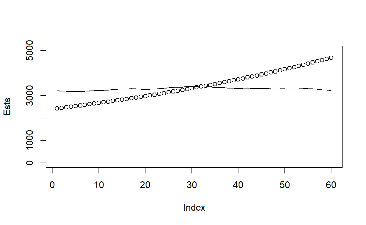
So we’re close to the right abundance of adults (trend is a bit off), but what about precision? Let’s approximate the variance-covariance matrix of the estimated parameters by taking the inverse of the negative Hessian (the second derivative of the likelihood function at the MLEs) and then get variance of abundance predictions using the delta method. Note that the vector \([N_1, N_2, N_3, \ldots, N_t]\) that we desire standard errors for are equivalent to \([\exp(p_1), \exp(p_1 + p_2), \exp(p_1+2p_2), \ldots, \exp(p_1 + (T-1)p_2)]\). The delta method requires taking the gradient of this vector relative to each of the parameters and then performing the following matrix operation:
Let’s plot our estimate with a log-based confidence interval and compare it to truth:
library(ggplot2)
Var_log = log(1+SE^2/Ests^2)
C = exp(1.96*sqrt(Var_log))
Plot_df = data.frame("Estimate"=Ests,"Truth"=Adults,"Lower"=Ests/C,"Upper"=Ests*C,"Year"=c(1:60))
ggplot(data=Plot_df)+geom_line(aes(x=Year,y=Ests),color="blue")+geom_line(aes(x=Year,y=Truth),color="black")+geom_ribbon(aes(x=Year,ymin=Lower,ymax=Upper),fill="blue",alpha=0.5)+ylim(c(0,max(Plot_df$Upper)))
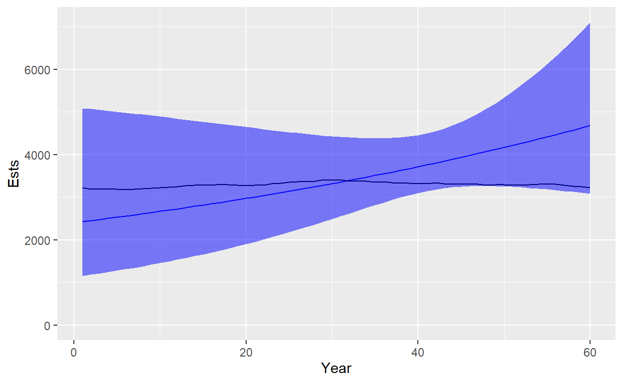
CV is low (<0.10) for the first year of sampling, but increases to about 0.2 at the end. Recall that sampling only occurred in the last 20 years of the time series, though estimates are available further back since we had to start the model a generation earlier.
If this were a “real” scoping study, we would certainly want to do a bit more simulation. Here is a short list of possible avenues:
- Repeat for a large number of simulations, investigating bias in absolute numbers and trend, confidence interval coverage, etc.
- Check to see if overall performance is better when trend parameter is fixed to zero
- Look at the impact of aging error. One could simulate aging error and see what happens if one assumes ages are known with certainty. Or, develop additional CKMR estimation models that permit estimation with imprecise aging or no aging (this requires a lot of integration and considerably complicates things)
- Look at the impact of imprecision and/or bias in survival and reproductive schedules
- Test what happens when mothers and their calves are likely to be sampled together (this is likely since sampled whales consist of those that are harvested by indigenous hunters). Or, we could retroactively eliminate this possibility by removing kin comparisons of adults with potentially dependent young.
- Look at model performance when half-sibs are included in the analysis