In this section, we shall attempt to explain the general approach to statistical inference for estimating abundance and demographic parameters from kinship data. This process largely the process of (1) formulating close-kin probabilities, and (2) scrunging them all into a pseudo-likelihood to make inference about demographic parameters. Although one can make modifications to these models that account for certain forms of imperfect genotyping, we assume here that kin finding proceeds without error.
Although it may be possible to formulate full likelihoods for pedigrees in certain circumstances, the approach outlined here is based on joint pseudo-likelihood, as originally outlined by Skaug [1] and Bravington et al. [2]. Under this framework, inference is made on the basis of pairwise comparisons between sampled animals, making the incorrect but simplifying assumption that genetic relationships between animals are independent. The resulting ``pseudo-likelihood" (so stated because it ignores the complicated nature of true pedigree structure) is then product-Bernoulli:
\[\begin{equation} L = \prod_i \prod_{j>i} \prod_k P_{ijk}^{y_{ijk}} (1-P_{ijk})^{(1-y_{ijk})}, \tag{1} \end{equation}\]
Here, \(i\) and \(j\) reference individuals, and the restriction \(j>i\) is to make sure we are not including cmoparisons twice. The subscript \(k\) denotes a type of kinship relationship (e.g., parent offspring, half-sibling), the \(P_{ijk}\) is the probability of a particular kinship relationship, and \(y_{ijk}\) is an indicator for whether animals \(i\) and \(j\) have this relationship or not. To conduct inference, one can maximize \(L\) relative to as set of parameter \(\boldsymbol{\theta}\) that determine \(P_{ijk}\) (or equivalently, minimize the negative log-likelihood). Such estimators are generally unbiased, and actually have reasonable variance properties provided that populations are large enough [2].
So, how should we go about specfiying the probabilities of kinship, \(P_{ijk}\)? These clearly differ based on the type of kinship relation that we’re considering. Although there are other ways of specifying probabilities (see e.g. [1]), we will rely on the notion of expected relative reproductive output (ERRO) as introduced in [2]. To illustrate how to use ERRO to calculate \(P_{ijk}\), let’s consider some specific examples
Mother-offspring pairs: age-known
Mothers and fathers often have different life histories, such that we’ll want to consider mother-offspring and father-offspring pairs separately. Without loss of generality, let’s let individual \(i\) be older than individual \(j\), and consider the probability that \(i\) is \(j\)’s mother. A Lexis diagram can help us think about the relationship between the two:
Here, \(b_i\) denotes the year of \(i\)’s birth, \(b_j\) is the year of \(j\)’s birth, \(d_i\) annd \(d_j\) are the years of their deaths (assuming lethal sampling, we know these), and \(a_i(b_j)\) is the age of individual \(i\) when \(j\) was born. The idea behind ERRO is to describe the expected reproductive output of \(i\) in year \(b_j\) relative to the total reproductive output of mothers in the population that year. More explicitly (and dropping the \(k\) subscript), \[\begin{equation*} P_{ij} = \frac{E[R_i(b_j)|{\bf z}_i,{\bf z}_j]}{E[R_+(b_j)|{\bf z}_j]}, \end{equation*}\] where
- \({\bf z}_i,{\bf z}_j\) are covariate vectors for animals \(i\) and \(j\) (sex, age, etc.)
- \(R_i(b_j)\) is reproductive output of animal \(i\) in \(b_j\), the year of \(j\)’s birth.
- \(R_+(b_j)\) is total reproductive output of the population in year \(b_j\)
How we specify \(R_i(b_j)\) and \(R_+(b_j)\) really depends on the underlying life history of the species in question. For example, if all mothers reach sexual maturity at the same age, and the expected reproductive output of all sexually mature mothers is the same (strong assumptions for sure), we could simply set \(E(R_i(b_j)) = 1.0\) and \(R_+(b_j)=N_{b_j}^F\), where \(N_{b_j}^F\) is the number of adult females in year \(b_j\). If we were only modeling mother-offspring pairs, we might attempt to estimate \(N_{b_j}^F\) when maximizing Eq. (1), or we might impose additional structure (e.g., \(N_{t}^F = N_0 \exp(kt)\), where \(\boldsymbol{\theta} = \{ N_0, k \}\) are estimated parameters). If, on the other hand, fecundity is age-specific (e.g., increases with age), we might set \(E(R_i(b_j)) = f_{a_i(b_j)}\) and \(R_+(b_j)=\sum_a N_{b_j,a}^F f_a\), where \(f_a\) is fecundity at age \(a\) (sensu Caswell 2001 [3]), and \(N_{b_j,a}^F\) is the number of age \(a\) females at time \(b_j\).
There are several points worth making here. The first is that we have just written \(P_{ij}\) in terms of adult abundance and fecundity parameters, which allows us to draw statistical inference about them using Eq. (1). The second is that parent-offspring close-kin analysis really only provides information on adult parameters, not juveniles. Third, when there is age-specific fecundity things get more complicated, and it becomes necessary to imbed an age-structured population model into the likelihood to calculate quantities such as \(N_{b_j,a}\). The model might omit juveniles entirely, or if additional information on juvenile survival is available these classes might be modeled as well. However, at minimum this formulation requires information on adult survival, which might be gained from simultaneous close-kin analysis of half-sibling pairs, or through auxiliary data like tagging or telemetry studies. Finally, we note that a recent study found that up to 62% of published studies that used matrix population models include errors [4]. When age-specific population models are imbedded within close-kin likelihoods, care should be taken in formulating the model so that it emulates life history of the species in question, including consideration as to whether reproduction is pre- or post-census, and whether survival needs to be included in fecundity terms. The authors of this primer are not immune from making such errors - you have been warned!
Mother-offspring pairs: ages uncertain
In most cases when assessing the age of an animal (e.g., through otoliths in fish, cementum annuli in mammals, or through epigenetics), there will be some uncertainty about the true age of the animal. Ideally this aging criterion would be calibrated to known age animals, so that, for instance, given some recorded age \(a^\prime\), we would know the probability of any true age \(a\), say \([a|a^\prime]\). This introduces uncertainty not only about age, but about the age of birth:
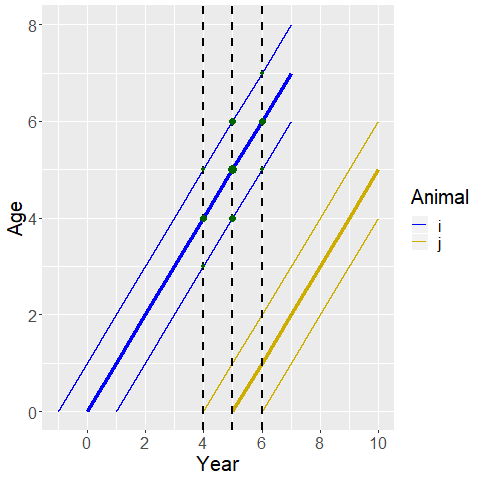
In the above diagram, we show the case where there is relatively minor aging error such that each animal is most likely the thicker line, but there is also a chance they are one year younger or older (the width of each line gives the relative probability that they are each age). In this case, there are 9 possibilities for the ages of the two animals, and we need to account for all of them. The relative probability of each pair of ages is represented by the width of the green circle at their intersection.
Mathematically this can be represented by integrating (in this case, summing) across all possible ages (or birthdays) of the two animals:
\[\begin{eqnarray*} P_{ij} & = & \sum_{b_j} \frac{\sum_{b_i} f_{b_j-b_i}[b_i|a_i^\prime]} {\sum_a N_{b_j,a}^F f_a} [b_j|a_j^\prime], \end{eqnarray*}\]
where, for instance, \([b_i | a_i^\prime]\) is the probability animal \(i\) was born in year \(b_i\) given it’s recorded age \(a_i^\prime\).
Let’s step back and think what we’ve learned here. First, we can adapt close-kin probabilities to account for imprecision in known ages. However, in order to do so we need information on the precision (and possible bias) of the aging criterion. By integrating over a wider and wider range of possible ages, is even possible to consider formulations for \(P_{ij}\) for animals where age is completely unknown. However, in general, precision will tend to decrease as aging errors increase (especially for adult survival estimated from half-siblings – more on that later). So, when designing a CKMR study, in addition to getting the genetic work right, and genotyping enough animals, one really has to give thought to making sure that one has reasonably precise aging criterion and that work has been done to allow calibration with true age (i.e., one should be able to estimate the probabilities \([b_i|a_i^\prime]\).
Maternal half-siblings, ages known
One of the things about close-kin analysis that seems like magic is the ability to estimate adult survival without ever having to sample one. This statement should come with a qualification, namely that we need to examine sufficient loci to discriminate half-siblings from the large mass of largely unrelated individuals and we need to have reasonably accurate ages. For the moment, let’s assume that ages are known with certainty. We’ll also assume that we know whether half-siblings share a mother or a father. Assuming there is sufficient mitochondrial haplotype diversity, we can often tell this because offspring inherit mitochondrial DNA from their mothers. So, if two half-siblings have the same mitochondrial haploytype, they are most likely related through their mother. If mito haplotype diversity is low, we could think about modeling \(P_{ij}\) using a mixture distribution where different haplotypes represent paternal half-siblings, but the same haplotype represents a mixture between paternal and maternal half-siblings. However, we’ll ignore that complication for now. Note, however, that in planning a close-kin study that uses half-siblings, researchers will often want to budget in extra funds for mitochondrial genotyping (in addition to normal SNP panels).
So, how should we formulate \(P_{ij}\) for maternal half-siblings? Let us suppose that individual \(i\) is born before \(j\), so that \(b_i < b_j\). According to Bravington et al. [2], the key is again to visualize things in terms of relative reproductive output. The prospective mother (let’s say \(d\)) must have given birth to animal \(i\) in year \(b_i\), survived \(b_j\), and then given birth to animal \(j\). Summing over possible mothers (the number of reproductively active females in year \(b_i\)), we have
\[\begin{equation*} P_{ij} = \sum_{d} \frac{E[R_d(b_i)]}{E[R_+(b_i)]} \frac{E[R_d(b_j)]}{E[R_+(b_j)]}. \end{equation*}\]
How this simplifies depends again on the biology of the species. Things are much easier in the case with knife-edge sexual maturity and when adult females are exchangeable (i.e. after maturity, females have homogeneous survival and fecundity), in which case we have
\[\begin{eqnarray*} P_{ij} & = & N_{b_i}^F \frac{1}{N_{b_i}^F} \frac{\phi_{b_i \rightarrow b_j}}{N_{b_j}^F} \\ & = & \frac{\phi_{b_i \rightarrow b_j}}{N_{b_j}^F}, \end{eqnarray*}\] where \(\phi_{b_i \rightarrow b_j}\) is the probability that an adult female survives from \(b_i\) to \(b_j\).
Things are more complicated when we have age-specific fecundity and survival, but after a little bit of math we can come up with something that looks like
\[\begin{equation*} P_{ij} = \sum_a N_{a,b_1} \frac{f_{a}}{\sum_{h} N_{h,b_1}f_{h}} \left( \prod_{y=b_1}^{b_2-1} S_{a+y-b_1} \right) \frac{f_{a+b_2-b_1}}{\sum_{h} N_{h,b_2}f_{h}}, \label{eq:halfsib} \end{equation*}\] where \(S_a\) is an annual survival probability for an age \(a\) female. Note that we have to account for uncertainty about the age of their prospective mother when they gave birth to the older individual. Things are even more complicated when we admit that ages are uncertain, but the point is that we can write them down - and thus conduct inference.
A final takeaway is that while parent-offspring pairs provide information on adult abundance (and, potentially, fecundity schedules), half-sibling relationships permit inference about adult abundance and adult survival.
Other kin relations: likelihood restrictions
In large, freely mixing populations, the probability of some relationships (e.g. full siblings) is exceedingly rare, provided that one does not compare individuals from the same cohort (assuming females produce >1 offspring). In fact, there are many reasons to not compare animals captured together, or that are born in the same year, since dependence in the fates of kin violates CKMR assumptions. It is also important to realize that half-siblings are genetically indistinguishable from a few other relationships (such as grandparent-grandchild or aunt-niece). Though aunt-niece is not likely to happen in practice, grandparent-grandchild certainly can if studies go on long enough. The obvious solution there is to omit comparisons from the likelihood where grandparent-grandchild is a possibility. For instance, if \(\alpha\) denotes the age at which animals become reproductive, we would omit comparisons for which \(b_j < b_i + \alpha\). Inference can then proceed using Eq. (1), but omitting contributions of comparison \(i\) and \(j\) when our requirements aren’t met. This may reduce sample sizes slightly, but it is a small cost to pay to avoid bias attributable to assumption violations. For certain life histories (e.g. territorial males with harems), some adaptation may eventually be needed to permit full siblings. However, to our knowledge such systems have yet to be examined for whether they would make sense for CKMR. It is unclear wither such systems are good candidates.
Assumptions
The preceding discussion brings to mind and important topic: what are the assumptions needed to conduct a CKMR analysis? These are well worth addressing before beginning a CKMR experiment! Here is a basic list:
- Accurate genotyping
- Appropriate population and sampling model
- No heterogeneity in kinship probabilities that can’t be explained by observed (or inferred) covariates
- Population is randomly sampled (Practically, this requires complete mixing or random sampling)
Several authors have investigated assumption violations. For instance, at the 2019 TWS/AFS conference, Eric Anderson demonstrated that false positives in kin matching can severely bias inference. Since there are so many comparisons being made, the implication is that many such errors could be made even in cases where they look small on paper.
A recent study also examined the random sampling assumption in spatially heterogeneous populations with dispersal limitation, and concluded (intuitively) that dispersal limitation coupled with spatially biased sampling can negatively bias estimates [5]. In such cases, spatially explicit models need to be formulated [e.g. 6], though these will often require higher sample sizes or additional data. For instance, one must make reproductive output spatially explicit, meaning that one must have a reasonable idea of how adults use space and dispersal occurs. Fortunately, there is information about dispersal in close-kin data that can help guide whether this is necessary or not [5].
Computing
For reasonably complicated close-kin estimation problems (e.g., including age-structure, aging error, etc.) it is extremely desirable to use a lower level language (such as C++) coupled with automatic differentiation to minimize the negative log-pseudolikelihood. Several popular alternatives that meet these criterion exist, including ADMB and TMB, with the latter recently having gained momentum in recent years. Built on templated C++ code, this platform gets the benefits of lower level languages without the need to completely learn a complex coding language like C++. The authors of this primer have at times used a combination of R, TMB, and C++ code linked to autodifferentiation libraries from TAPENADE, depending on the application. In our Examples, we include a mixture of R and TMB applications.
Regardless of software choice, note that a major obstacle in evaluating the pseudo-likelihood is that there are a total of \(k * {n \choose 2}\) pairwise comparisons between animals, where \(n\) is the number of genetic samples. So, for \(n=10,000\), we have nearly 50 million potential calculations to evaluate the likelihood a single time if we just used brute force. In practice, a couple of suggestions can help speed up computation. First, instead of calculating \(P_{ijk}\) separately for each comparison, it makes sense to factor the likelihood by grouping comparisons that have the same covariate values (e.g., age, year sampled). This will substantially decrease the number of times \(P_{ijk}\) has to be calculated. One can also use these groupings to define binomial (as opposed to Bernoulli) likelihood components in Eq. (1). Finally, the number of times the likelihood needs to be evaluated should decrease substantially when using autodifferentiation.