Design
Conducting a CKMR experiment can be an expensive endeavour. Although genotyping costs have come down substantially in recent years, by the time one factors in the cost of panel development and processing individual samples, one can easily reach a price tag ranging from the tens of thousands to millions of dollars for the genetics alone (depending upon the size of the sample). And that is before factoring in the costs of sampling and analysis. We thus highly recommend conducting a CKMR scoping analysis prior to actually collecting and analyzing data. The goal of a scoping study is to determine whether CKMR is likely to be an appropriate for the population of interest and that resulting estimates will have adequate precision to meet monitoring objectives.
Scoping exercises should consider both biology and sampling. Certain reproductive biologies are simply not amenable to CKMR (e.g. asexual reproduction), while other populations may be too small (e.g., \(<500\) or too large (e.g., \(>100,000,000\)) to make CKMR feasible. In other species, behavior may make some of the assumptions underlying existing CKMR models unlikely to be met. For instance, group living species may exhibit inbreeding that makes kin finding prone to error; dispersal limitation and/or mixed migration strategies may also bias traditional CKMR estimators [2] depending on how sampling is conducted.
Sampling considerations include the number of genetic samples collected, as well as the temporal and spatial distribution of sampling. For instance, in a scoping study of Atlantic bluefin tuna, [2] examined the influence of spatially biased sampling under mixed migration strategies and determined that traditional CKMR models would result in biased estimates, but that spatially explicit models would produce accurate inference (unfortunately at the cost of higher sample sizes).
Sample size: basic rules of thumb
In their seminal paper, [3] developed some basic rules of thumb for sample sizes needed for CKMR inference. First, the number of genetic samples required to generate abundance estimates with a desired level of precision is proportional to the square root of adult abundance. This means that if it takes \(n=1000\) samples from a population to produce adequate precision for a population of \(N=20,000\), it will take \(n=\sqrt{200000}/\sqrt{20000}*1000 \approx 3200\) samples to produce the same level of precision for a population of \(N=200,000\). This is quite fortunate, as it means that populations can be quite large before CKMR is impractical. Second, they suggest shooting for a minimum of 50 kin pairs to reach a target CV of 0.15 in simple parent-offspring-pair (POP) models; if sampling is conducted more or less instantaneously (as opposed to a multi-year monitoring program) and there are roughly equal numbers of juveniles and adults, this translates into needing roughly \(n = 10\sqrt{N}\) genetic samples [3]. Unfortunately, sample sizes need to be higher than this if considering a multi-year study, or ones that need to estimate an increased number of parameters to account for biological realism or to accommodate aging error. In my experience, it is a mistake to rely on rules of thumb in these situations as they will tend to be overly optimistic. Fortunately we can rely on simulation experiments (or “scoping studies”) to determine the sample size we should shoot for to arrive at a desired level of precision.
Structure of a scoping study
Ideally, a scoping study should involve biologists, geneticists, and statisticians. If preliminary genetic information is available, it can be used to judge the number of markers that will be needed to reliably enumerate specific relationships (e.g., HSPs, POPs) and to determine whether there is sufficient mitochondrial haplotype diversity to discriminate maternally and paternally related kin pairs (for HSPs). Biologists can weigh in on aspects of life history that may likely affect inference, which can then be accounted for in potential simulation studies. Finally, assuming that CKMR still seems potentially useful, statisticians (or quantitatively astute ecologists) can perform simulation studies to assess precision under various sampling scenarios. These studies can also consider different CKMR models that either do or do not account for relevant life history or sampling features (i.e., to see whether simpler CKMR models are robust to likely assumption violation).
Simulation studies include development of one or more operating models, and one or more estimation models, with performance diagnostics tabulated for each combination:
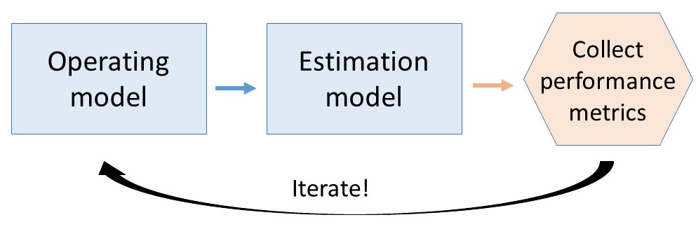
Operating models
In the context of CKMR, an operating model defines the population size and structure, specifies annual (or other time step) population dynamics, and determines genetic relationships between individuals. Two types may be used: population-based model or individual-based models.
Population-based models simply generate time series of stage-specific abundances (as with Leslie-matrix models), with the number of kin-matches generated as random realizations dependent on the number of samples and the probability of observing a different type of kin-pair. In this version of an operating model, the probabilities of kin pairs are based on the concept of relative reproductive output, as specified in e.g., [3]. The potential danger here is that the operating model will often be more or less identical to the estimation model and if coding errors exist they may be propagated into both models and are potentially undiscoverable. Another limitation is that it will be difficult to assess potential CKMR assumption violations. Nevertheless, this may be a useful first step in determining precision when all assumptions are met.
In serious applications, we recommend using forward-time, individual-based operating models. These should be doable to construct for most populations, although extremely large populations may have lengthy simulation times [4]. Two software packages are currently available to facilitate individual-based pedigree simulations, both in the R computing environment [5]: fishsim and CKMRpop [4]. These packages allow features such as movement between demes, age- and sex-specific mortality and fecundity schedules. Typically, one will need to specify initial age- and sex-specific abundance values (“founders”), run the simulation for a burn-in period until founders are all dead (since these do not have recorded parents), and then run the simulation for an additional “monitoring” period. Both packages keep track of parental relationships, and include algorithms for population sampling and for determining kin pairs among the sampled individuals.
Estimation models
Estimation models calculate CKMR pseudo-likelihoods given a specified model, demographic parameters (such as adult abundance or survival), and data. As part of the estimation process, the CKMR pseudo-likelihood is maximized (technically it is the negative log-pseudo-likelihood which is minimized) using a numerical optimization routine (such as “nlminb” or “optim” in R) by sequentially adjusting demographic parameter values until an optimal solution is reached. Optimized parameter values (pseudo-MLEs) serve as point estimates for model parameters, with associated numerical routines providing standard errors. Often, derived parameters (functions of parameters) will also be of interest, standard errors for which can be obtained via the delta method [7]. Relatively simple estimation models can be programmed directly in R, but with increasingly complicated ones (e.g., employing aging error or other loop-heavy pseudo-likehoods) it can be beneficial to program them in a lower level language that has auto-differentiation capabilities (e.g., ADMB, TMB). Some examples of estimation models are provided here.
Although not explicity part of an estimation model, it may also be worthwhile to examine performance with different types of data restrictions. For instance, eliminating comparisons of mothers and offspring that are sampled in the same year can help eliminate assumption violations (in this case, dependence of fates that can positively bias abundance estimates). Or, eliminating half-sibling comparisons for individuals whose times of sampling are greater than some threshold value to eliminate possible contamination by grandparent-grandchild pairs (these two categories have the same expected number of shared genes). Such restrictions will presumably make inferences more accurate, at the cost of slightly reduced precision.
Evaluating performance
Performance of CKMR estimators depend on what quantity is of interest to biologists and managers. Sample size requirements, for instance, will be much lower if one wishes to calculate average adult abundance over a long time period than it will be if interest focuses on abundance in the most recent year. Since data do not give much information in the final year of the study, so we will usually need to be build in population trend parameters in some form into the estimation model. Estimates will be less precise with a linear trend parameter than a more flexible form (e.g., via a quadratic or smoothing spline).
Once a metric is decided upon, the usual statistical summaries can be used to evaluate performance: e.g., percent relative bias, mean squared error, anticipated CV, and confidence interval coverage. Ideally, an estimator would meet a desired level of precision, display low bias, and have confidence interval coverage close to nominal. Exploring estimator performance when the operating model has increasingly realistic biology and sampling intracacies can be a good way of examining the robustness of an estimating model, in the sense that one can examine potential bias and confidence interval coverage when standard CKMR assumptions are not met. For instance, [1] examined performance of a spatially homogeneous CKMR model when the true biology included dispersal limitation and when sampling was spatially restricted.
Examples
A simple design example, patterned off the biology of beluga whales in northern Alaska, is presented here.