In this example, we attempt to deploy a CKMR model where there isn’t any information on ages. For simplicity, we’ll assume a knife-edge model for reproductive output that applies equally to each sex. Further, we’ll assume that all sampling is of adults.
In this case, when we compare each sample to another, the only information we have to go on is the year of sampling. For POP analysis, we must treat two cases for each comparison, one in which A is the mother of B, and another where B is the mother of A, integrating (summing) over possible ages of each animal while accounting for the probability that each animal is of a certain age. This actually requires that we have some model for survival (in a POP-only analysis, this could be treated as a constant or modeled with a prior distribution) so that, e.g., the probability of an animal being 5 years old is greater than it being 50 years old. For HSPs, we’ll need to again integrate over the possible ages of the animals being compared (if survival is age-dependent, we’d also need to integrate over possible ages of the parent).
Let’s consider the case where individuals become adults at age 3, and reach a survival probability of 0.8 at age 2. We’ll use CKMRpop (and spip by extension) to simulate data - see the beluga design example for more information on installing this software.
library(CKMRpop)
library(dplyr)
pars <- list()
pars$`max-age` <- 20
pars$`fem-surv-probs` <- pars$`male-surv-probs` <- c(0.5, 0.7, rep(0.8,18))
pars$`fem-prob-repro` <- c(rep(0,3),rep(1,17)) #probability of reproduction
pars$`male-prob-repro` <- pars$`fem-prob-repro`
pars$`fem-asrf` <- rep(2,20)  #if they reproduce, expected # offspring
pars$`male-asrp` <- rep(1,20)  #each reproductively mature male has same expected repro output
#pars$`offsp-dsn` <- "binary"  #override default neg. binomial dist. for litter size
pars$`sex-ratio` <- 0.5
Now we’ll set up some initial conditions and specify the length of the simulations. We’ll base the age structure of founders on stable age proportions computed using Leslie matrices, as calculated via the leslie_from_spip functionality in CKMRpop. We’ll also set up the simulation to run for 70 years assuming that sampling is conducted over the last 10 years (we need to go back three generation times from the start of sampling to ensure grandparents all have parents).
pars$`number-of-years` <- 70
# this is our cohort size
cohort_size <- 1000
# Do some matrix algebra to compute starting values from the
# stable age distribution:
L <- leslie_from_spip(pars, cohort_size)
pars$`initial-males` <- floor(L$stable_age_distro_fem)
pars$`initial-females` <- floor(L$stable_age_distro_male)
pars$`cohort-size` <- "const 1000"
samp_start_year <- 61
samp_stop_year <- 70
pars$`discard-all` <- 0
pars$`gtyp-ppn-fem-post` <- paste(
samp_start_year, "-", samp_stop_year, " ",
paste(c(0,0,0,rep(0.04, pars$`max-age`-3)), collapse = " "), #sampling proportion 4% / year of adults only
sep = ""
)
pars$`gtyp-ppn-male-post` <- pars$`gtyp-ppn-fem-post`
set.seed(2020) # set a seed for reproducibility of results
spip_dir <- run_spip(pars = pars) # run spip
slurped <- slurp_spip(spip_dir, 2) # read the spip output into R
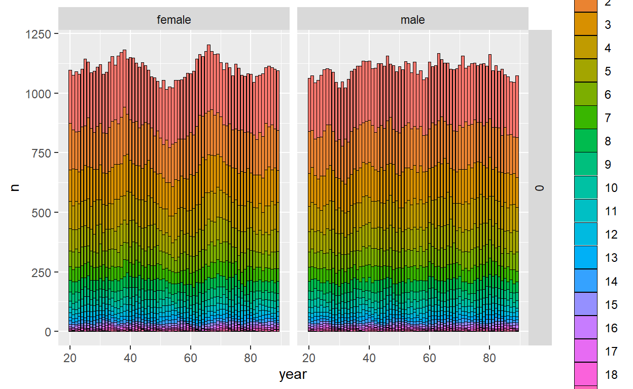
ggplot_census_by_year_age_sex(slurped$census_postkill)
Let’s take a look at the number of kin pairs we ended up sampling:
nrow(slurped$samples)
[1] 442 crel <- compile_related_pairs(slurped$samples)
relat_counts <- count_and_plot_ancestry_matrices(crel)
relat_counts$highly_summarised
# A tibble: 5 x 3
  dom_relat max_hit     n
  <chr>       <int> <int>
1 FC              1   497
2 A               1   411
3 Si              1   165
4 PO              1    76
5 GP              1    33
So, we have 165 half-siblings, 76 parent-offspring pairs, and 33 grandparent-grandchild pairs. One issue when we don’t have ages is that it’s going to be difficult to impose constraints that prevent us from confusing grandparent-grandchild pairs from half-sibling pairs. Let’s see if there are any other metrics that might work… specifically, difference in sampling times.
  crel$time_diff = rep(NA,nrow(crel))
  for(i in 1:nrow(crel))crel$time_diff[i]=abs(crel$samp_years_list_1[[i]][1]-crel$samp_years_list_2[[i]][1])
  GP_time_diff = crel[which(crel$dom_relat=="GP"),]$time_diff
  HS_time_diff = crel[which(crel$dom_relat=="Si"),]$time_diff
  summary(GP_time_diff)
   Min. 1st Qu.  Median    Mean 3rd Qu.    Max.
0.000 2.000 4.000 4.061 6.000 8.000 summary(HS_time_diff)
   Min. 1st Qu.  Median    Mean 3rd Qu.    Max.
   0.00    1.00    2.00    2.63    4.00    8.00
Okay, so it looks like half-sibs are a bit more likely to be encountered closer in time than grandparent-grandchild pairs, but there is still substantial overlap. With the life history we’re considering here, there is thus no real reliable way to tell them apart. Let’s concentrate on POPs instead.
To model POPs, let’s once again boil things down to sufficient statistics. In this case, we’ll order each comparison so that the animal encountered first is “animal 1” and the animal encountered later is “animal 2” - but we’ll need to know the time (year) each animal was sampled (\(t_i\)). If reproductive schedules differed among sexes, we’d also need to know the sex of each animal, but we’re not going to consider that complication for here. So, the sufficient statistics will be \(y_{t_1,t_2}\) and \(n_{t_1,t_2}\), which are the number of parent-offspring pairs observed in years \(t_1\) and \(t_2\), and the number of PO comparisons made for years \(t_1\) and \(t_2\), respectively. Note that through all of this, we’re only using first captures (CKMRpop by default uses live sampling, but we’ll just use the first of these to mimic lethal sampling). Here’s some code to calculate the sufficient statistics:
  n_indiv = nrow(slurped$samples)
  n_samp_t = samp_stop_year - samp_start_year + 1
  y_tt = n_tt = matrix(0,n_samp_t,n_samp_t)
  POPs = crel[which(crel$dom_relat=="PO"),]
  for(i in 1:nrow(POPs)){
    samp_t1 = POPs$samp_years_list_1[[i]][1]-60
    samp_t2 = POPs$samp_years_list_2[[i]][1]-60
    if(samp_t1>samp_t2)y_tt[samp_t2,samp_t1]=y_tt[samp_t2,samp_t1]+1
    else y_tt[samp_t1,samp_t2]=y_tt[samp_t1,samp_t2]+1
  }
  for(i1 in 1:(n_indiv-1)){
    for(i2 in (i1+1):n_indiv){
      samp_t1 = slurped$samples$samp_years_list[i1][[1]][1]-60
      samp_t2 = slurped$samples$samp_years_list[i2][[1]][1]-60
      if(samp_t1>samp_t2)n_tt[samp_t2,samp_t1]=n_tt[samp_t2,samp_t1]+1
      else n_tt[samp_t1,samp_t2]=n_tt[samp_t1,samp_t2]+1
    }
  }
Okay, so we have the data. So now we have to specify the probability that each POP comparison results in a match - which is a function of relative reproductive effort (which in turn depends on adult population size), accounting for uncertainty in the age of each animal. Since we don’t have the ages, we need to have a model that probabilistically says something about the age of each animal at the time of capture; in absence of other information, it is proportional to the cumulative survival of living to a particular age. Let’s assume that we know adult survival perfectly (i.e., it is 0.8 for all adults). In this case, the probability that a sampled animal is a particular age is given by \(\pi\), pre-calculated here:
Now, let’s write a function to calculate the negative log pseudo-likelihood given our data, as a function of a single unknown adult abundance parameter (which will be on the log scale) - we’ll start by assuming a model where adult abundance remains constant over time.
  get_p <- function(it1,it2,Pi,n_a,N_t){
    cur_p = 0
    for(ia1 in 4:n_a){  #we're assuming only adults are sampled (so 0,1,2 yr olds are not possible)
      for(ia2 in 4:n_a){
         ib1 = it1-ia1+n_a
         ib2 = it2-ia2+n_a
         if((ib2-ib1)>2 & ib2<(it1+n_a)){ #animal 1 is old enough to be parent and dies (is sampled) after ind. 2 is born
           cur_p = cur_p + Pi[ia1-3]*Pi[ia2-3]*2/N_t[ib2]
         }
         if((ib1-ib2)>2 & ib1<(it2+n_a)){ #animal 2 is old enough to be parent, etc.
           cur_p = cur_p + Pi[ia1-3]*Pi[ia2-3]*2/N_t[ib1]
         }
      }
    }
    cur_p
  }

  nlpl = function(pars,data){
    log_p = function(p) log(p+(p==0))
    N_t = rep(100+exp(pars[1]),data$n_t)  #include lower bound to prevent weird rel repro effort
    nll = 0
    rem_tt = data$n_tt - data$y_tt
    for(it1 in 1:10){
      for(it2 in it1:10){
        cur_p = get_p(it1,it2,data$Pi,data$n_a,N_t)
        nll = nll - data$y_tt[it1,it2] * log_p(cur_p) - rem_tt[it1,it2] * log_p(1-cur_p)
      }
    }
    nll
  }
This is a fairly simple binomial likelihood… let’s optimize it and make sure we’re getting a reasonable answer.
  pars_CKMR = log(1000) #initial values for log(adult abundance-100)
  data = list(n_tt=n_tt,y_tt=y_tt,Pi=Pi,n_a=20,n_t=30)
  nlpl(pars_CKMR,data=data)
[1] 622.9099 Opt = nlminb(pars_CKMR,nlpl,data=data)
#calculate variance and plot results
Adults = rep(0,10)
for(iyr in 61:70)Adults[iyr-60]=sum(slurped$census_postkill$female[which(slurped$census_postkill$year==iyr & slurped$census_postkill$age>3)])+sum(slurped$census_postkill$male[which(slurped$census_postkill$year==iyr & slurped$census_postkill$age>3)])
Ests = 100+rep(exp(Opt$par[1]),10)
VC = solve(numDeriv::hessian(func=nlpl,x=Opt$par,data=data))
grad=exp(Opt$par[1])
SE = sqrt(grad * VC * grad)
CV = SE / Ests
library(ggplot2)
Var_log = log(1+SE^2/Ests^2)
C = exp(1.96*sqrt(Var_log))
Plot_df = data.frame("Estimate"=Ests,"Truth"=Adults,"Lower"=Ests/C,"Upper"=Ests*C,"Year"=c(1:30))
ggplot(data=Plot_df)+geom_line(aes(x=Year,y=Estimate),color="blue")+geom_line(aes(x=Year,y=Truth),color ="black")+geom_ribbon(aes(x=Year,ymin=Lower,ymax=Upper),fill="blue",alpha=0.5)+ylim(c(0,max(Plot_df$ Upper)))
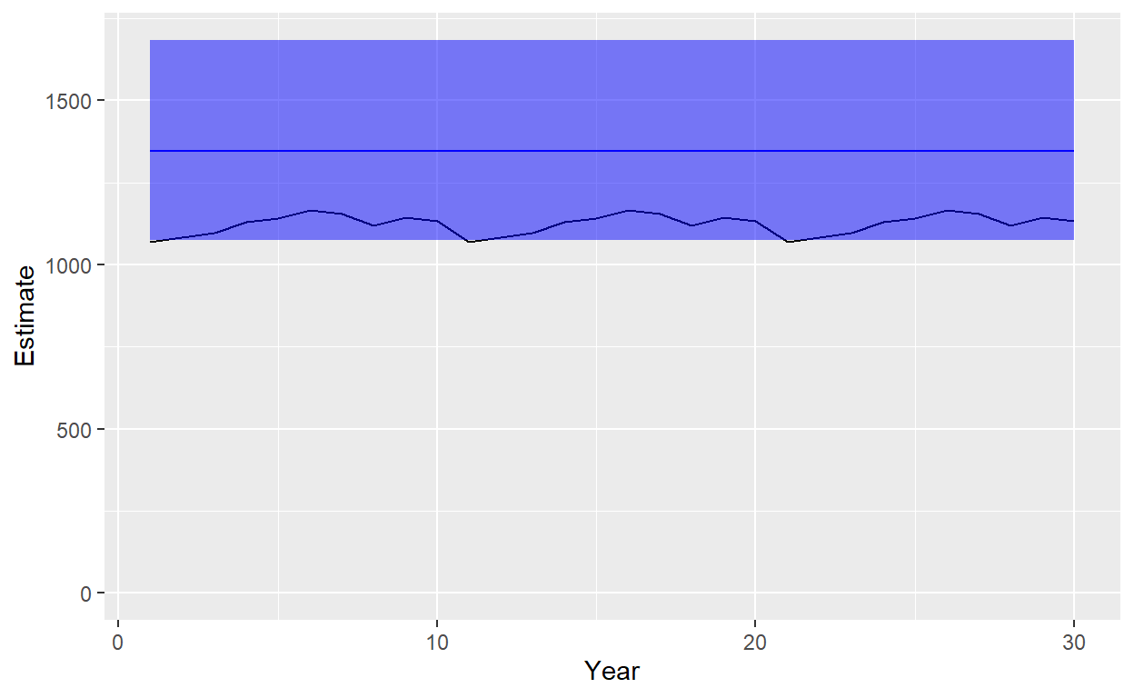
So, our time-constant abundance model produced an estimate that was slightly high for this particular simulation, but includes true abundance for most of the time series within the 95% confidence interval. CV in this case is actually pretty good, at 0.1146602. Let’s try refitting this with a linear trend model for abundance.
  nlpl = function(pars,data){
    log_p = function(p) log(p+(p==0))
    N_t = (100+exp(pars[1]))*exp(c(0:(data$n_t-1))*pars[2])
    nll = 0
    rem_tt = data$n_tt - data$y_tt
    for(it1 in 1:10){
      for(it2 in it1:10){
        cur_p = get_p(it1,it2,data$Pi,data$n_a,N_t)
        nll = nll - data$y_tt[it1,it2] * log_p(cur_p) - rem_tt[it1,it2] * log_p(1-cur_p)
      }
    }
    nll
  }

  pars_CKMR = c(log(1000),0) #initial values for log(adult abundance-100), r
  data = list(n_tt=n_tt,y_tt=y_tt,Pi=Pi,n_a=20,n_t=30)
  nlpl(pars_CKMR,data=data)
[1] 622.9099 Opt = nlminb(pars_CKMR,nlpl,data=data)
#calculate variance and plot results
Adults = rep(0,10)
for(iyr in 61:70)Adults[iyr-60]=sum(slurped$census_postkill$female[which(slurped$census_postkill$year==iyr & slurped$census_postkill$age>3)])+sum(slurped$census_postkill$male[which(slurped$census_postkill$year==iyr & slurped$census_postkill$age>3)])
Ests = (100+exp(Opt$par[1]))*exp(Opt$par[2] * c(0:(data$n_t-1)))
VC = solve(numDeriv::hessian(func=nlpl,x=Opt$par,data=data))
Grad = matrix(0,2,data$n_t)
Grad[1,1]=exp(Opt$par[1])
Grad[2,1]=0
for(i in 2:data$n_t){
Grad[1,i]=exp(Opt$par[1]+(i-1)*Opt$par[2])
Grad[2,i]=(i-1)*exp(Opt$par[1]+(i-1)*Opt$par[2])
}
SE = sqrt(diag(t(Grad) %*% VC %*% Grad))
CV = SE / Ests
Var_log = log(1+SE^2/Ests^2)
C = exp(1.96*sqrt(Var_log))
Plot_df = data.frame("Estimate"=Ests,"Truth"=Adults,"Lower"=Ests/C,"Upper"=Ests*C,"Year"=c(1:30))
ggplot(data=Plot_df)+geom_line(aes(x=Year,y=Estimate),color="blue")+geom_line(aes(x=Year,y=Truth),color ="black")+geom_ribbon(aes(x=Year,ymin=Lower,ymax=Upper),fill="blue",alpha=0.5)+ylim(c(0,max(Plot_df$ Upper)))
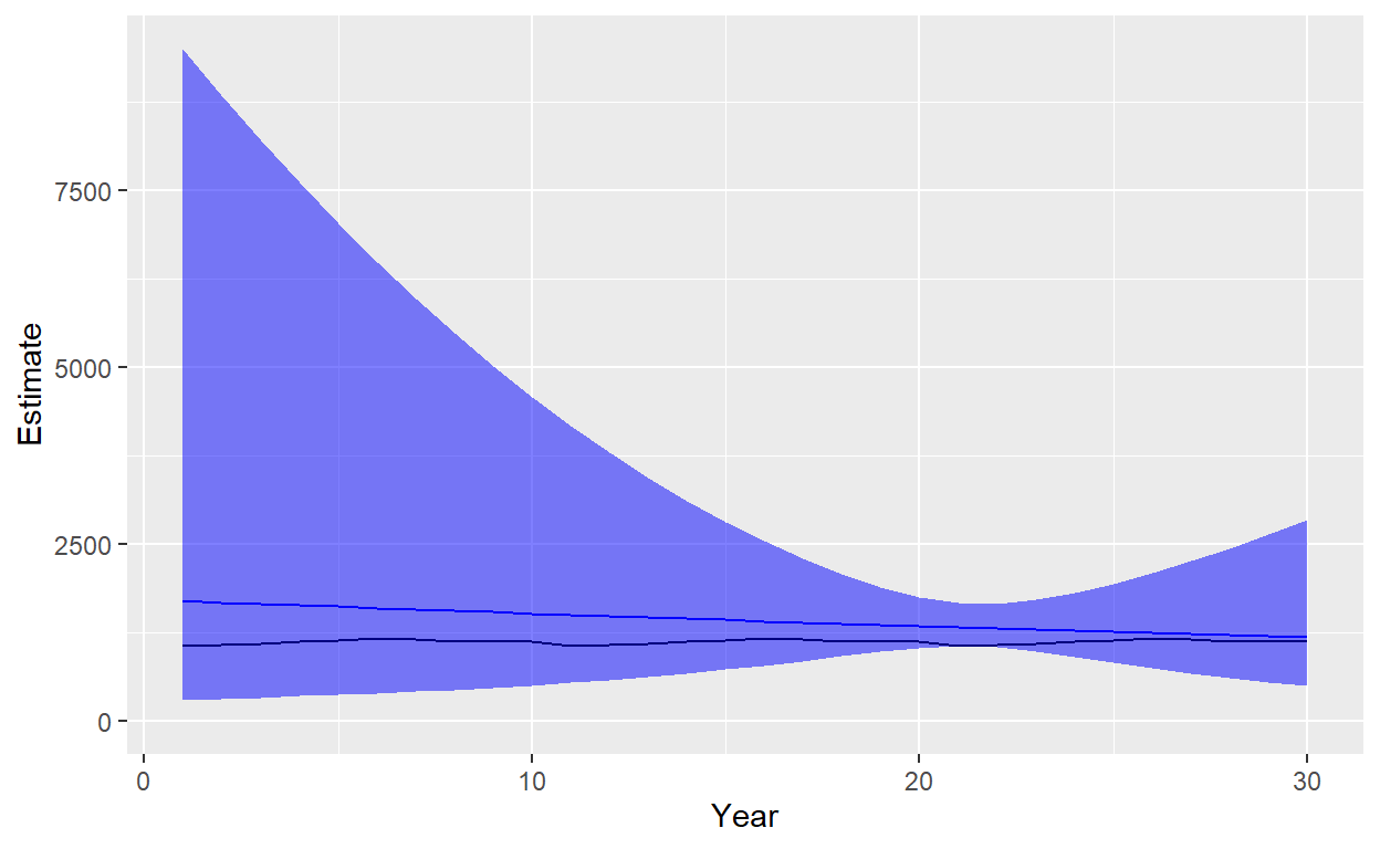
So we’re estimating that the population is slightly decreasing, but the trend estimate has a 95% CI which considerably overlaps zero. We can see that the estimated precision is best near the beginning of data collection (CV near 0.12), but considerably worse at the end of the time series (CV 0.47). However, we were able to estimate abundance even without ages! It is worth noting that we assumed we knew adult survival - precision would only decrease if we incorporated uncertainty about its value (e.g., by inclusion of a prior distribution rather than a fixed known value).